

At a glance
Two new functions, GROUPBY and PIVOTBY, allow you to create summary report layouts like PivotTables. But unlike PivotTables, the reports update automatically if the data changes.
A single formula creates a two-dimensional report that summarises a dataset.
I recommend using a formatted table as the data source for these functions. Formatted tables have the advantage of automatically expanding as data is added to the table, which means the report will always be up to date.
The example data
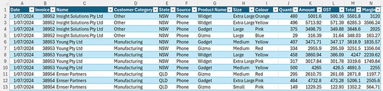
Figure 1 shows the sales data used to demonstrate these new functions. The table is named tblSales.
GROUPBY function
This new function is the simpler of the two and requires three arguments to create a summary report.
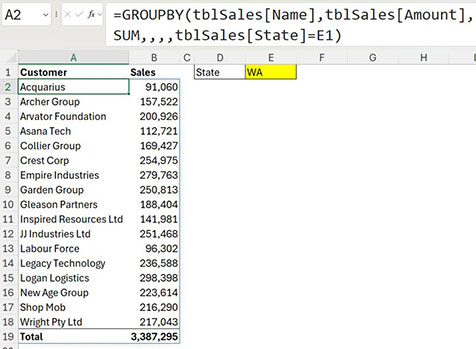
Figure 2 shows the single function in cell A2 that spills down and across to create a summary report.


This report lists the unique entries from the State column and sums and totals the values from the Amount column for the report.
The third argument allows the user to select the function to use in the report — see Figure 3.
Formatting
Unfortunately, the spill range does not spill formats. The reports need to be formatted manually. The remaining examples will be formatted.
Multiple columns
The GROUPBY function can summarise more than one column. See an example in Figure 4.

I have split the formula over two lines in the Formula Bar to create a better image.
Since the Customer Category column is next to the State column within the table you can create a single reference to refer to them both as shown in the formula. Notice the extra set of square brackets around the column names and the colon between the column names.
What if the columns are not next to each other?
There are at least two functions that combine separate columns.

HSTACK function
This function combines columns of data into a single range. Figure 5 shows a summary report by Source and Size.

CHOOSECOLS function
This function combines columns based on the column number within a range. This creates a shorter formula, but it is not as descriptive as HSTACK. Figure 6 shows the same report from Figure 5 created using CHOOSECOLS.
The CHOOSECOLS function is combining the 6th and 8th columns from the table.
Totals
The default setting for GROUPBY is to show the overall total at the bottom of the report. The fourth argument handles the total positioning and whether to include subtotals. Totals can be omitted or shown at the top or bottom. Figure 7 shows two examples.

Conditional formatting
Totals are typically formatted differently to detail rows. Conditional formats can be used to apply a different format to the total rows no matter where they appear in the report. See examples in Figure 8.


The Conditional Formatting settings for the report are shown in Figure 9. The rule applies the bold font with top and bottom borders when cells in column B are blank. The $B2 reference ensures all three columns in the range refer to column B.
This conditional format works for two or more level reports. This assumes there are no blank cells in the Size column in the data table.
Filtering
PivotTables also offer filtering. The seventh argument of the GROUPBY function handles filtering. In Figure 10, the report shows customers for WA only.
Slicer filtering
It is possible to filter the GROUPBY report using a slicer, just like a PivotTable. A slicer is a graphical filter user interface. Slicers can be used to filter formatted tables.
The formula solution is long and complex and is explained in more depth in the companion video. Figure 11 has an example.

Multiple value columns
The GROUPBY report can also return more than one calculation. The new PERCENTOF function automates the percentage of total calculations that are possible in PivotTables. HSTACK is used to include more than one function.
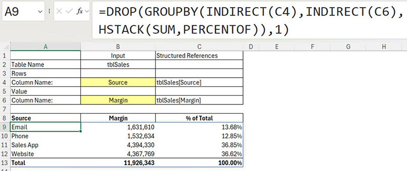
Figure 12 has an example of the PERCENTOF function.

DROP function
As Figure 12 shows, the GROUPBY function includes the function names in the first row when returning more than one function. That heading row can be removed with the DROP function.
See Figure 13 for an example.

Flexible reports
PivotTables can be changed easily. Changing the GROUPBY function is a manual process that involves editing the formula. Flexibility can be added to a GROUPBY report by using the INDIRECT function.
The INDIRECT function converts text into a reference that can be used by a formula. That reference can refer to a cell, range, formatted table or a range name. This allows cell entries to control and change the report generated by the GROUPBY function.
See Figures 14 and 15.
The user can select the columns for the report using the two yellow drop-down cells.

PIVOTBY function
This function works the same as the GROUPBY function for rows but also includes columns for the report. It has 11 arguments. The first four arguments are required, the others are optional.
Figure 16 shows a basic PIVOTBY report.

The Customer Category is listed in the rows and the State is shown in the columns.
Function arguments
The same arguments for totals and filters apply to PIVOTBY. The extra arguments relate to settings for the columns for the report.
Handling dates
PivotTables make it easy to group dates into months, quarters and years. You can use the TEXT function to achieve date grouping in these two new functions.
The TEXT function converts dates into text strings. Unfortunately, text is sorted alphabetically in GROUPBY and PIVOTBY. This means that month names will be listed in alphabetic order starting with April and August. A special custom number format code can avoid this issue.

Figure 17 shows an example.
The code "yyyy-mm-mmmm" in the TEXT function displays the full year, the two numeric digits for the month, followed by the full month name. This structure ensures the dates are grouped and displayed in the correct sequence.
Performing extra calculations
Calculating a margin percentage can’t be done within the GROUPBY function. A LET function can capture the GROUPBY result and add a column to it calculating the margin percentage.
Figure 18 shows an example calculating the margin percentage.

The formula in Figure 18 is explained in the companion video.
Sorting
GROUPBY and PIVOTBY both have sorting arguments, and these are covered in the companion video.
These new functions offer many different reporting options. In many cases they can replace PivotTables.
The companion video and Excel file will go into more detail to demonstrate these techniques.

